The end of the year is almost here and since next year is a multiple of 5 (2020) the new updated World Magnetic Model (WMM) has been released on December 10th. If you didn’t knew why Annex 4 mentions that the magnetic variation needs to be reviewed every 5 years at least now you have an idea why this period may have been chosen.

From Annex 4 Definition
Magnetic variation. The angular difference between True North and Magnetic North.
Note.— The value given indicates whether the angular difference is East or West of True North
From Annex 4 Standards
2.15 Magnetic variation
2.15.1 True North and magnetic variation shall be indicated. The order of resolution of magnetic variation shall be that as specified for a particular chart.
2.15.2 Recommendation.— When magnetic variation is shown on a chart, the values shown should be those for the year nearest to the date of publication that is divisible by 5, i.e. 1980, 1985, etc. In exceptional cases where the current value would be more than one degree different, after applying the calculation for annual change, an interim date and value should be quoted.
Note.— The date and the annual change may be shown.
2.15.3 Recommendation.— For instrument procedure charts, the publication of a magnetic variation change should be completed within a maximum of six AIRAC cycles.
2.15.4 Recommendation.— In large terminal areas with multiple aerodromes, a single rounded value of magnetic variation should be applied so that the procedures that service multiple aerodromes use a single, common variation value.
Calculation of single locations
So let’s see how much the magnetic variation has changed for one specific place on the earth.
Let’s take this aerodrome declared variation on the eAIP from FMMI (Antanarivo International Airport), its magnetic variation published for 2015 says 15°W so let’s do the calculation for Epoch 2020.0 (1 January 2020)

We will be using the single point calculator from NOAA and first lets do a check on the value for 2015, the calculator is easy to use but since WMM is valid for 5 year periods only I will use one of the other available model IGRF to do the check getting the 15°W value.
To do the calculation let’s use the ARP of the airport and its height AMSL. The model changes with height but it wont make a huge difference.

Now let’s change the value to WMM and 1 January 2020


So you can see that in five yearst the change isn’t that much as the change per year is minimal, it usually takes a decade for shifting one degree in most parts of the world and since we just show a one degree resolution it doesn’t really show easily. Also as these are models you can check that the IGRF predicted a change of 1 minute 53 seconds per year while the new WMM model is predicting a change per year of four minutes and 20 seconds.
Basically in about two more years the change would be enough to cross the 30 minutes mark to change from 15°W to a 16°W magnetic declination
The following map shows the declination isolines where the change is in minutes per year

Calculation of Isogonals
One specific case is that in some aviation charts we are supposed to show the isogonals e.g. [ENR Chart]
Extract from Annex 4
7.7 Magnetic variation
Recommendation.— Isogonals should be indicated and the date of the isogonic information given
From Annex 4
Isogonal. A line on a map or chart on which all points have the same magnetic variation for a specified epoch
For this I will create a sample using WMM2020 and Epoch 2020.0 which corresponds to 1 January 2020 and I will choose an interesting location in earth, in this case Magadascar using eAIP ASECNA . In the larger version you can see it has the isogonals every 2 degrees

First step I will draw the FIR based on the publication of the eAIP, unfortunately I think there is no AIP/AIXM dataset available. I could use other sources but just for fun I will create a CSV file copy paste the coordinates from the eAIP file and import in QGIS. Unfortunately the eAIP has some weird format to separate lat/lon with dashes and other stuff that requires a bit more of handling


Loading the CSV points with QGIS


For doing the isogonals I will get the minimum bounding geometry of the FIR and add a buffer to it just to have some extra margin. To buffer I will use Laborde Projection which encompass Magadascar


For this example I will add 10NM buffer around the bounding box, but first I will save the calculated bounding box in the projected coordinate system (PCS) and then apply the buffer


After having the buffer I returned the map to EPSG 4326 (WGS84) to get the extent in lat/lon

Note: Actually to get the isogonals you just need to set the grid interval and that can be taken directly from the screen or estimated, in this blog post I just wanted to combine other things to introduce several GIS functions. You can skip all the above and just turn the grid and select the appropriate boundary coordinates. Due to the size of the FIR the 10 NM buffer is irrelevant


Now using the grid function from the WMM NOAA website and adding all the parameters we can download in several formats, I am using CSV as its easy to read with any spreadsheet and can be loaded easily in QGIS. One of the parameters you need to input is elevation, I will use 0ft because honestly the difference is insignificant and I got numbers, as we round anyway the average magnetic declination difference between flying at 40000ft AMSL and assuming 0ft AMSL in this region is 0.06 degrees


The file that get’s downloaded looks like this initially
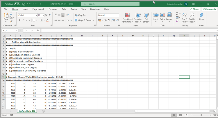
Some modification to be used in QGIS, basically remove the header and add custom name to fields and save as CSV as a separate file (I never overwrite the original raw data for traceability)

Now time to load in QGIS and check how it all fits


So now we have loaded the data of the declination for every degree and we just need to do an interpolation to get the isogonals, to do this using QGIS and the processing framework TIN interpolation, use the layer as the extent


Its time to extract contours


Now I will add an extra field to know when a contour is major or minor, I will consider major if its divisible by 5, for this I will use the modulo operator using math you will see that if a number is divisible by 5 then the remainder shall be 0

Final Version

Want to learn more or want to get in touch? Visit also www.antoniolocandro.com and use the contact form there for services you may require


2 Comments
Naing Min Latt · December 18, 2019 at 6:46 pm
Thanks a lot
Jacquelyne Mcintyre · January 4, 2020 at 3:15 am
some really interesting information, well written and generally user genial.